Contemporary music analysis with machine learning tools
Pablo E. Riera
Laboratorio de Acústica y Percepción Sonora y Laboratorio de Dinámica Sensomotora.
Universidad Nacional de Quilmes.
TALLER SOBRE APLICACIONES MATEMÁTICAS Y COMPUTACIONALES A LA MÚSICA
Buenos Aires - 14 al 18 de noviembre de 2016
Facultad de Ciencias Exactas y Naturales - Universidad de Buenos Aires
Convocado por el Centro Latinoamericano de Formación Interdisciplinaria (CELFI)
Contemporary Music, Electroacoustic Music and Experimental Music
“This listening experience is characterised by a new vision of time (i.e. atemporal, static, periodic), space (i.e. multi-channels diffusion and sculptural musical design), musical evolution (non-narrative and extended) and repetition (generation of hypnotic effects and a listening ‘in accumulation’). These characteristics form an (ec)static listening environment, where the musical material is static (atemporal, non-narrative) and the listening attitude is ecstatic (free to explore and move through the dimensions of sound).”
Wanke, R. (2015). A Cross-genre Study of the (Ec) Static Perspective of Today’s Music. Organised Sound, 20(03), 331-339.
Scope
- Contemporary, electroacusctic and experimental music
- Focus on timbre
Situation
- How to compare timbres?
- Different criteriums for grouping sound and making timbre spaces
- Timbre spaces aren't unique
Attempts
- For a specific musical piece, try to obtain a timbre space that allows to explore and go through the palette of sounds
Timbre spaces
Sounds of musical instruments may be positioned in a low dimensional space with dimensions asociated to acoustic attributes.
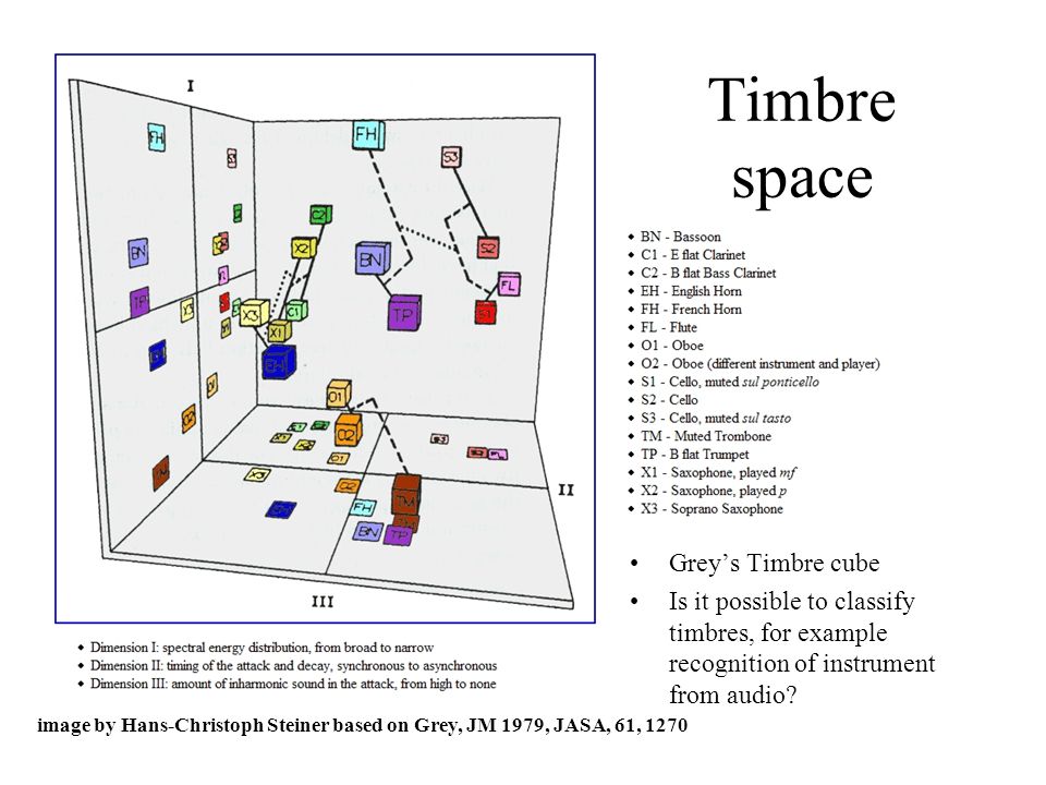
Grey, J. M. (1977). Multidimensional perceptual scaling of musical timbres. the Journal of the Acoustical Society of America, 61(5), 1270-1277

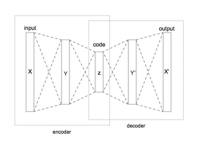
Unsupervised Learning with Autoencoders
- Spectrum -> Encoding -> Low dimensional neuronal representation -> Decoding -> Spectrum

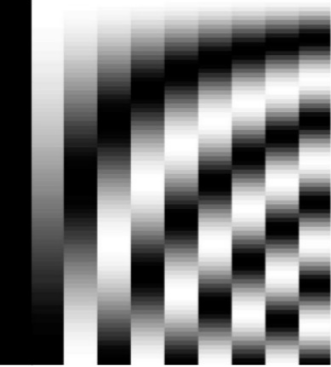
Discrete Cosine Transform basis
Partiels (Grisey 1975)
%%HTML
<video width="640" height="640" controls>
  <source src="figs/Partiels/spectrogram_video.mp4" type="video/mp4">
</video>
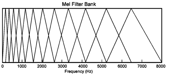
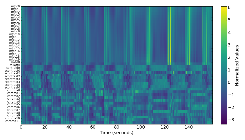
Features
%%HTML
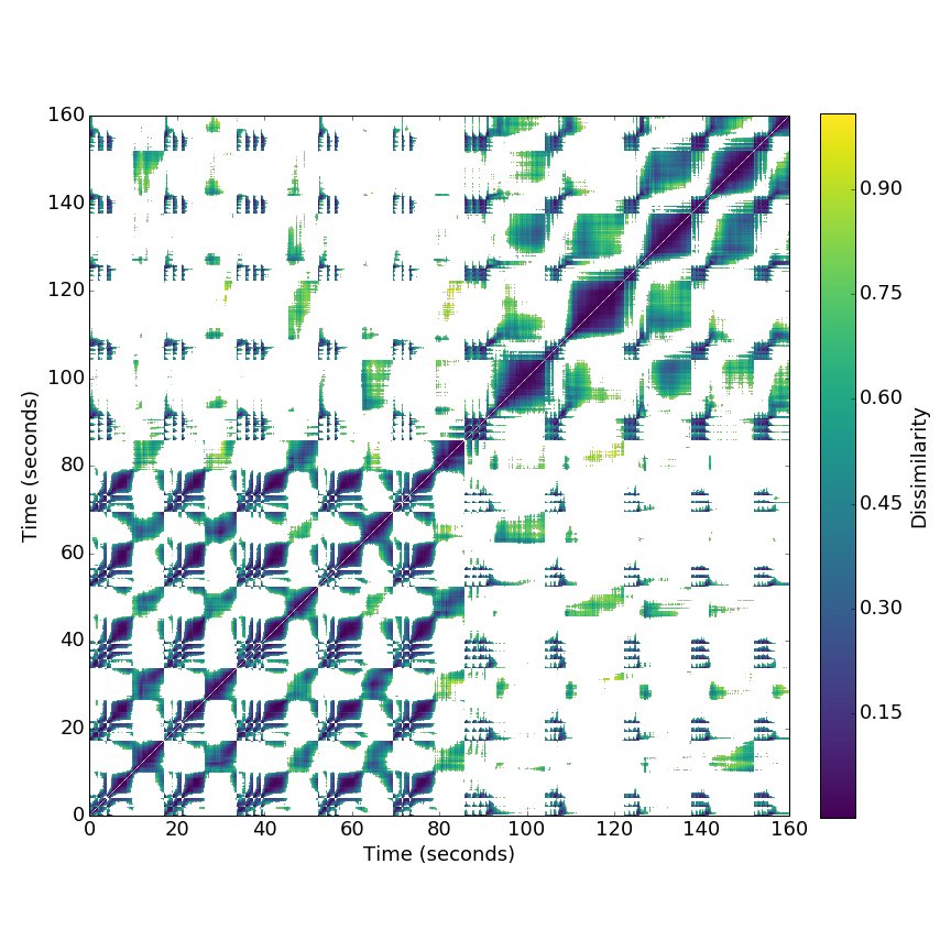
<H1> Recurrence - Partiels Grisey (1975) </H1>
<video width="640" height="640" controls>
<source src="figs/Partiels/recurrence_video.mp4" type="video/mp4">
</video>
%%HTML
<video width="640" height="480" controls>
  <source src="figs/Partiels/mds_video.mp4" type="video/mp4">
</video>
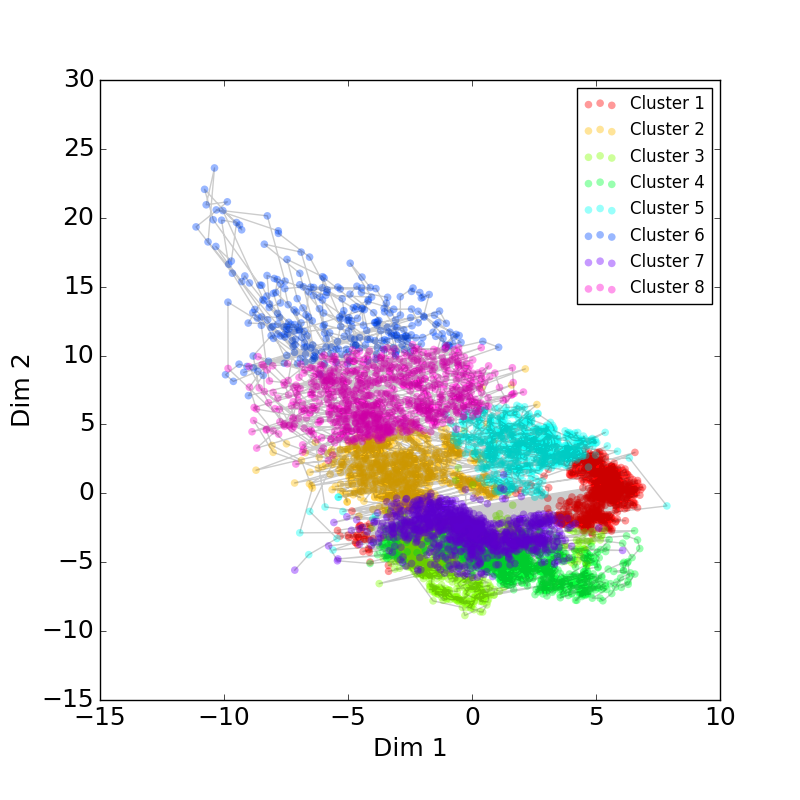
Clustering K - Means and Spectral
display(htmlimage(['figs/Partiels/mds_kmeans_labels.png'],512))
# ,'figs/Partiels/mds_spectral_labels.png'
# display(htmlimage('figs/Partiels/mds_kmeans_labels.png.png',512))
Clustering with K - Means
# import pickle
# sr = 44100
# with open('../mir/pickles/Partiels_data.pickle', 'rb') as handle:
#     s = pickle.load(handle)

# X = s['Xpca']
# n_clusters=X.shape[1]
# labels = s['kmeans_labels']
# print(s['name'])
# path = 'figs/'
# for i in range(n_clusters):
#     fname = s['name']+'/kmeans_cluster_'+str(i)+'.mp3'
#     display(audiofile(filename=path+fname))
path = 'figs/Partiels'
for i in range(8):
    fname = '/kmeans_cluster_'+str(i)+'.mp3'
    display(audiofile(filename=path+fname))
Following a path in timbre space
Wessel, D. L. (1979). Timbre space as a musical control structure. Computer music journal, 45-52.
Sorting the time axes with first principal component
display(audiofile(filename='figs/Partiels/pca_sorted.mp3'))
Traversing the recurrence graph
display(audiofile(filename='figs/Partiels/orderdfs.mp3'))
Timbre in the brain: Auditory cortical response
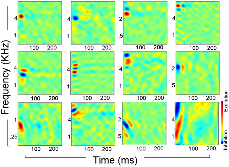 Patil, K., Pressnitzer, D., Shamma, S., & Elhilali, M. (2012). Music in our ears: the biological bases of musical timbre perception. PLoS Comput Biol, 8(11)
Autoencoders
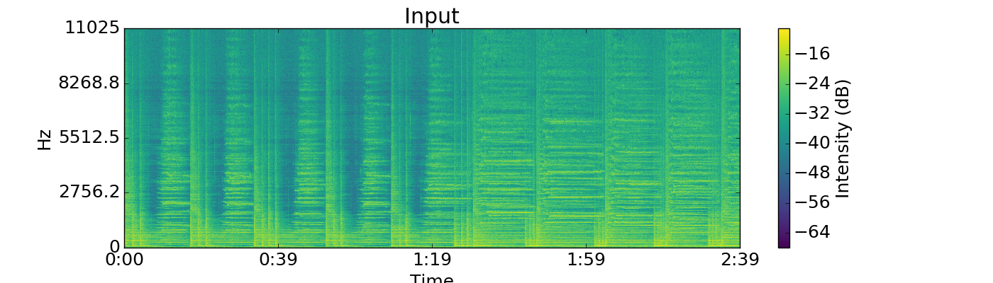
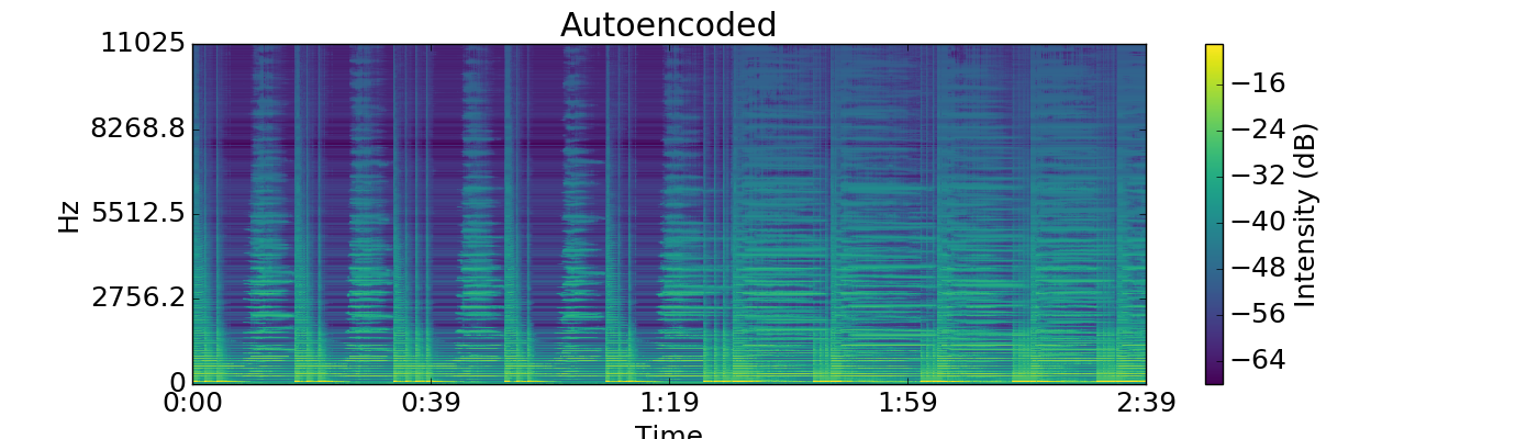
display(audiofile(filename='figs/Autoencoder/naeoutput_8.mp3'))
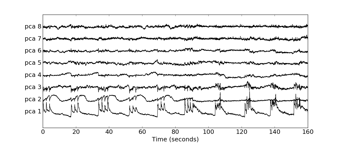
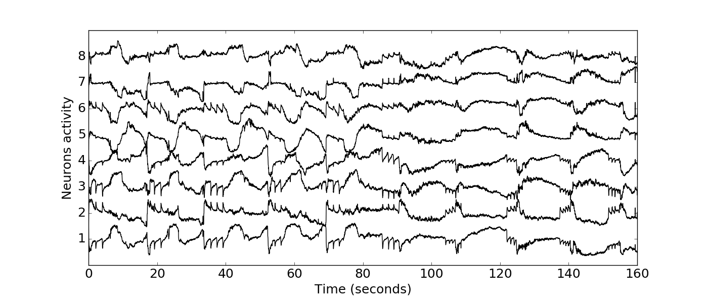
Code Layer Neuronal activity
Spectral receptive fields in the encoded layer
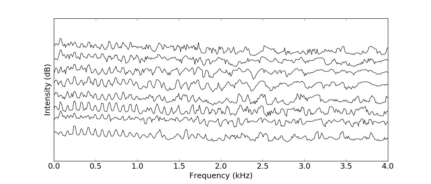
display(audiofile(filename='figs/Autoencoder/zpath_8.mp3'))
%%HTML
<video width="640" height="512" controls>
  <source src="figs/Partiels/mdsz_video.mp4" type="video/mp4">
</video>
display(htmlimage(['figs/Partiels_nae_inner_layer/recurrence_cosine.png'],512))
Autoencoder Neural activity
- Autoencoder with 8 neurons bottleneck learns reasonably well because overfits the small dataset
- Multidimensional scaling space is substantially different from Audio Descriptor results, but not acoustically correlated
Agradecimientos
- Matias Zabaljauregui, Alejo Salles, Martín Miguel, Andrés Babino, Alma Laprida